Image Segmentation

Segmentation of the image to be explained into “superpixels” is usually the first step when using LIME to explain an image classifier’s output.

For this, both the original implementation and VisuaLIME rely on methods implemented in scikit-image. The scikit-image documentation contains an excellent introduction to and discussion of the segmentation methods available in VisuaLIME.

This guide discusses why image segmentation is necessary, how to choose a method to use, and how to find suitable parameters for it.

Why?

Digital images processed by computer vision models, such as photographs, are usually stored as raster graphics. They are represented as multidimensional arrays, where each entry in the array corresponds to a so-called pixel. The pixels are the individual points that taken together make up the image.

VisuaLIME works with 8-bit RGB(A) images, where each pixel is described by three (four) values between 0 and 255:

• Red

• Green

• Blue

• Alpha (the transparency/opacity)

Thus, each image is represented by a 3-dimensional array of shape (image_height, image_width, 3) or (image_height, image_width, 4), respectively.

While it makes sense to store and process images this way, when it comes to explaining machine-learning models, this format is problematic.

On the one hand, even a small thumbnail image with a size of 224 x 224 pixels will be represented by an array with a total of 150,528 entries. Analyzing how each of these values contributes to a model’s output quickly becomes computationally infeasible. (It’s no coincidence that most deep learning computer vision models only work with relatively small images and aim to reduce the amount of data they need to process within the first few layers.)

On the other hand, and that’s arguably the even bigger problem, human’s do not think and talk about images in pixels. Instead, they see shapes, areas, objects, details. If we’re looking to generate explanations that humans can understand and comprehend, they need to reflect that.

Thus, the first step in creating a visual explanation with LIME is to divide the image into segments (also called “superpixel”). Image segmentation is a standard procedure in digital image processing and many methods have been developed over the years.

Selecting a method

Which segmentation method is suitable in your case depends on the images that you’re processing. For example, images that contain both small details and large areas of unimportant background will require a method that can pick up on that and create segments of vastly different size. So you’ll need to get a representative set of examples, try a couple of different methods, and iterate your way to a suitable set of parameters.

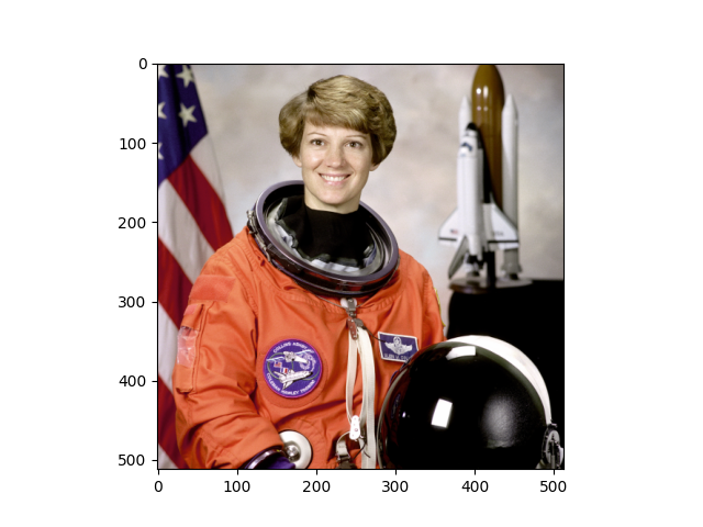
For this guide, we’ll use the portrait of astronaut Eileen Collins that is included as an example image in scikit-image. (You can download this guide and replace the following lines with your own image loading code.)

import matplotlib.pyplot as plt
from skimage import data

image = data.astronaut()
plt.imshow(image)
plt.show()

felzenszwalb

TODO

• Tends to be close to human perception: Segments can have vastly different size and number of segments will vary a lot between images

• Only one parameter to tune (scale), but if you’re off you might get an unintelligible maze

from skimage.segmentation import felzenszwalb, mark_boundaries

fig, ax = plt.subplots(2, 2, figsize=(10, 10), sharex=True, sharey=True)

for i, scale in enumerate((1, 10, 100, 1000)):
    ax[i // 2, i % 2].set_title(f"scale={scale}")
    ax[i // 2, i % 2].imshow(
        mark_boundaries(
            image,
            felzenszwalb(image, scale=scale, sigma=0.5, min_size=50),
        )
    )
plt.show()

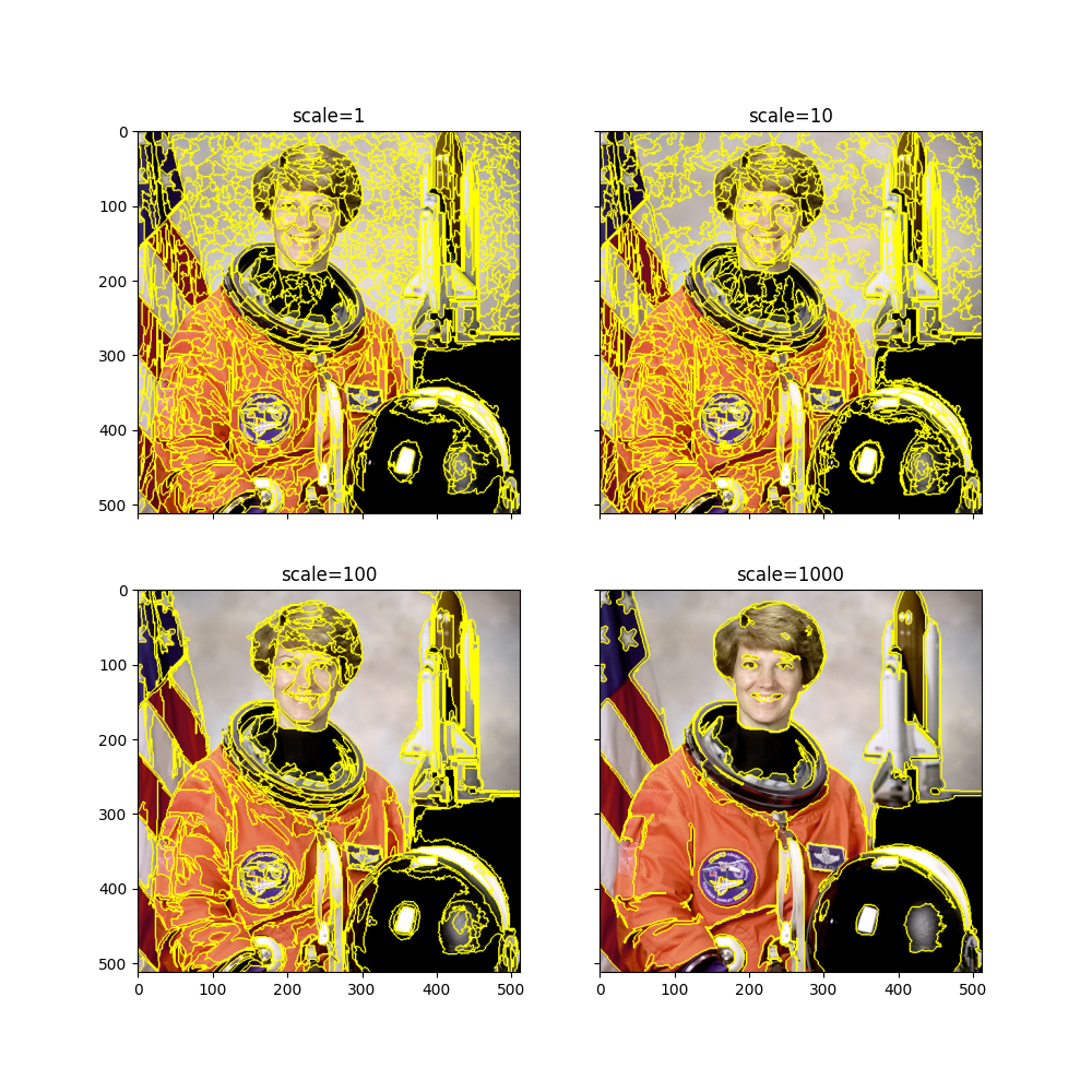
• In general, this method is the easiest to tune, and it is rather fast.

Note

If you’re using this method to segment your images, the cosine similarity between the samples generated by visualime.lime.generate_samples() (the default choice) is not a good distance measure as the segments are of very different size.

You’ll have to calculate the distances on an image-level (e.g., using visualime.lime.compute_distances()) and pass a distances array to the subsequent steps.

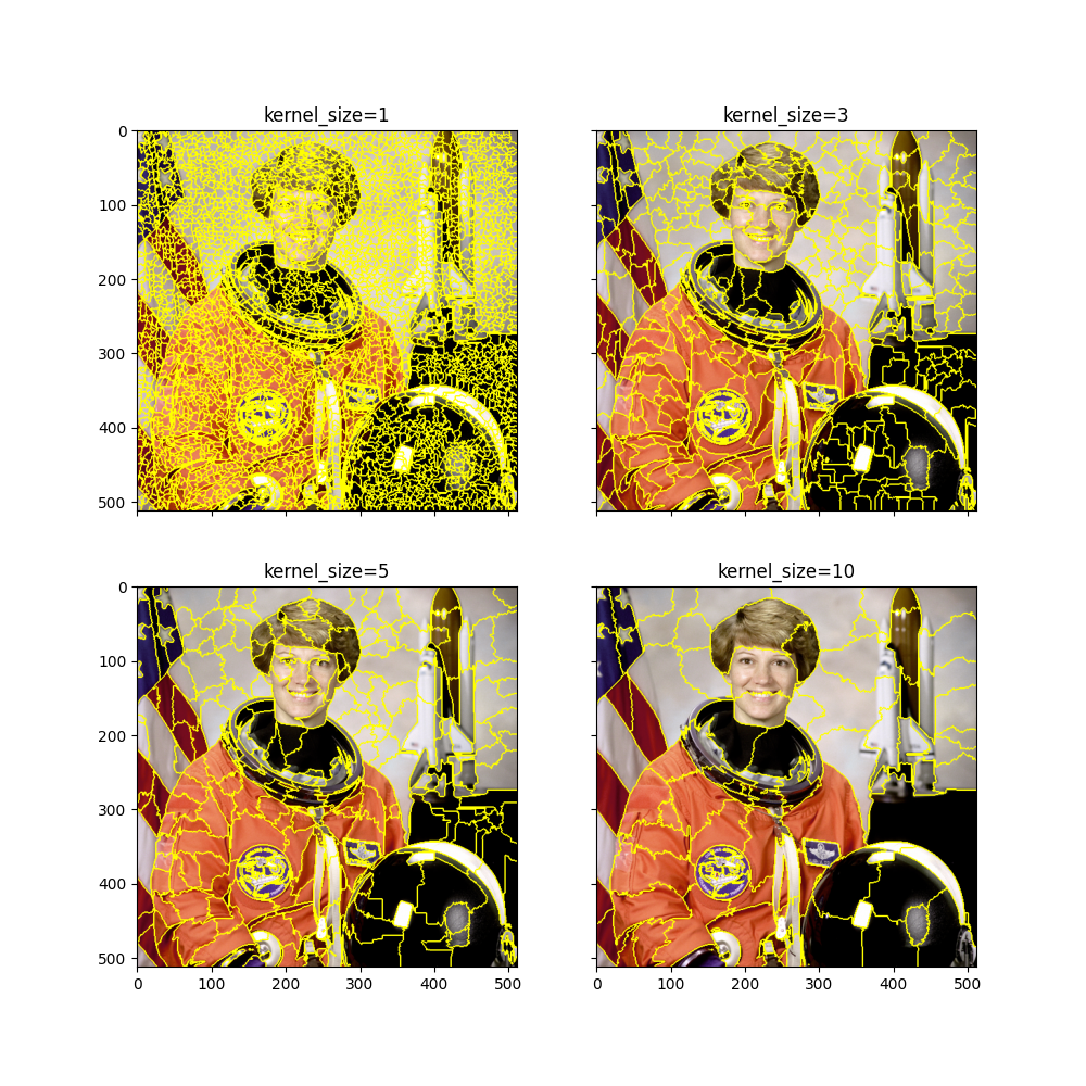
quickshift

TODO

from skimage.segmentation import quickshift

fig, ax = plt.subplots(2, 2, figsize=(10, 10), sharex=True, sharey=True)

for i, kernel_size in enumerate((1, 3, 5, 10)):
    ax[i // 2, i % 2].set_title(f"kernel_size={kernel_size}")
    ax[i // 2, i % 2].imshow(
        mark_boundaries(
            image,
            quickshift(image, kernel_size=kernel_size, max_dist=10, ratio=0.5),
        )
    )
plt.show()

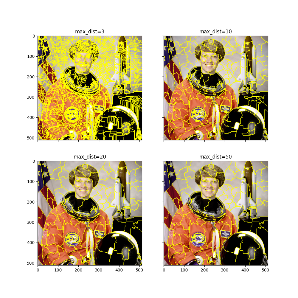
max_dist

fig, ax = plt.subplots(2, 2, figsize=(10, 10), sharex=True, sharey=True)

for i, max_dist in enumerate((3, 10, 20, 50)):
    ax[i // 2, i % 2].set_title(f"max_dist={max_dist}")
    ax[i // 2, i % 2].imshow(
        mark_boundaries(
            image,
            quickshift(image, kernel_size=5, max_dist=max_dist, ratio=0.5),
        )
    )
plt.show()

slic

TODO

• Need to define the number of segments

• Can control regularity of segments with compactness parameter, leads to segments of similar size in a grid

watershed

TODO

• Need to define the number of segments

• Can control regularity of segments with compactness parameter, leads to segments of similar size in a grid

VisuaLIME has a helper function that computes the gradient.

Tuning a segmentation method

TODO